Parameter Estimation Guide

Most baseflow separation methods in baseflowx require at least one parameter -- typically a recession coefficient -- and some require two. Choosing these parameters appropriately is essential: a poorly calibrated filter can produce baseflow estimates that are physically implausible, even if the filter itself is mathematically sound. This guide walks through the standard approaches for estimating each parameter, with code examples showing the recommended workflow.

Recession coefficient estimation

The recession coefficient \(a\) (sometimes written \(k\) or \(K\)) characterizes the rate at which aquifer storage drains into the stream during periods of no recharge. It appears in nearly every recursive digital filter in baseflowx -- Eckhardt, Chapman-Maxwell, Boughton, Willems, and others all require it. Physically, a high recession coefficient (close to 1.0) indicates a slowly draining aquifer with large storage, while a lower value indicates a flashier response. For daily streamflow data, typical values fall in the range 0.90 to 0.99.

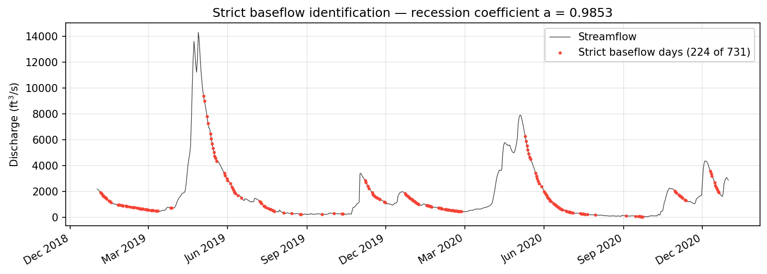
baseflowx estimates the recession coefficient in two steps. First, strict_baseflow() identifies the timesteps that are unambiguously part of a baseflow recession, applying derivative-based heuristics to exclude rising limbs, storm peaks, and their immediate aftermath. Second, recession_coefficient() examines the ratio of the centered derivative to the discharge at those strict baseflow points, sorts those ratios, and selects the 5th percentile value. The 5th percentile is used rather than the median or mean because it targets the steepest uncontaminated recessions, which best represent the aquifer's intrinsic drainage rate without interference from residual quickflow.

The mathematical relationship is as follows. Given the centered finite difference \(dQ = (Q_{t+1} - Q_{t-1})/2\) and the concurrent discharge \(cQ = Q_t\), the function computes \(dQ/cQ\) for all strict baseflow points, selects the value at the 5th percentile of the sorted (descending) ratios, calculates \(K = -cQ/dQ\) at that index, and returns \(a = e^{-1/K}\).

import baseflowx

data = baseflowx.load_sample_data()
Q = data['Q']

# Step 1: identify strict baseflow periods
strict = baseflowx.strict_baseflow(Q)

# Step 2: fit the recession coefficient
a = baseflowx.recession_coefficient(Q, strict)
print(f"Recession coefficient: {a:.4f}")

Recession coefficient estimation for the Fish River dataset, showing the distribution of dQ/Q ratios at strict baseflow points and the 5th-percentile fit.

The strict_baseflow() function accepts a quantile parameter (default 0.9) that controls how aggressively it excludes post-event periods. Setting a higher quantile relaxes the definition of a "major event," retaining more points but potentially including some with residual quickflow influence. For most applications the default is appropriate.

If the catchment is affected by ice or snowpack, pass a boolean mask via the ice argument to exclude those periods from the recession analysis. Winter discharge records in cold regions often reflect ice dam formation and breakup rather than aquifer dynamics, and including them can bias the recession coefficient estimate.

BFImax for the Eckhardt filter

The Eckhardt (2005) filter requires two parameters: the recession coefficient \(a\) and the maximum baseflow index \(\text{BFI}_\text{max}\). While \(a\) characterizes the temporal dynamics of aquifer drainage, \(\text{BFI}_\text{max}\) controls the upper bound on the long-term baseflow fraction. Getting \(\text{BFI}_\text{max}\) right is critical because the Eckhardt filter's output is highly sensitive to this parameter -- it directly governs how much of the total streamflow volume is attributed to baseflow.

There are three principal approaches to estimating \(\text{BFI}_\text{max}\), each with different data requirements and assumptions.

Approach 1: literature values from Eckhardt (2005)

Eckhardt (2005) proposed default \(\text{BFI}_\text{max}\) values based on hydrogeological setting. These remain widely used as a starting point when no site-specific calibration data are available:

Hydrogeological setting	\(\text{BFI}_\text{max}\)
Perennial streams with porous aquifers	0.80
Ephemeral streams with porous aquifers	0.50
Perennial streams with hard-rock aquifers	0.25

These values should be treated as order-of-magnitude guidance rather than precise calibration targets. Real catchments exhibit substantial variability even within the same hydrogeological class, and the "right" value for a particular site may differ from the tabulated default by 0.1 or more. Nevertheless, the Eckhardt defaults provide a defensible starting point for exploratory analyses.

import baseflowx

data = baseflowx.load_sample_data()
Q = data['Q']

strict = baseflowx.strict_baseflow(Q)
a = baseflowx.recession_coefficient(Q, strict)

# Use a literature value for a perennial stream with porous aquifer
b = baseflowx.eckhardt(Q, a, BFImax=0.80)

Approach 2: annual maximum BFI

The maxmium_BFI() function estimates \(\text{BFI}_\text{max}\) from the streamflow record itself by computing the baseflow index for each year of data and taking the maximum. The logic is that in the driest year -- the one with the least storm activity -- the observed BFI most closely approximates the true baseflow fraction, since there is less quickflow to confound the estimate.

The function first runs a backward-recursive baseflow separation using the Lyne-Hollick filter output and the recession coefficient, then computes annual BFI values. If the maximum annual BFI exceeds 0.9, the function falls back to the overall BFI (total baseflow divided by total discharge), as values near 1.0 typically reflect artifacts rather than genuine hydrogeology.

from baseflowx.estimate import maxmium_BFI

# b_LH is the Lyne-Hollick baseflow, a is the recession coefficient
b_LH = baseflowx.lh(Q)
BFImax = maxmium_BFI(Q, b_LH, a)
print(f"Estimated BFImax: {BFImax:.3f}")

b = baseflowx.eckhardt(Q, a, BFImax=BFImax)

If date information is available, pass it via the date argument to compute true calendar-year BFI values rather than dividing the record into 365-day blocks:

import numpy as np

dates = data['dates']
# Convert dates to a pandas-like structure with a .year attribute,
# or use numpy datetime handling
BFImax = maxmium_BFI(Q, b_LH, a, date=dates)

Approach 3: CMB calibration

When concurrent specific conductance data are available for even a portion of the discharge record, the Conductivity Mass Balance method provides a physically grounded calibration target. The calibrate_eckhardt_from_cmb() function runs CMB over the overlap period, computes the resulting BFI, and returns it as the \(\text{BFI}_\text{max}\) for use with the Eckhardt filter on the full record. This approach combines the physical rigor of the tracer method with the temporal coverage of the digital filter.

from baseflowx.tracer import calibrate_eckhardt_from_cmb

# Q_sc and SC are arrays for the period with conductance data
result = calibrate_eckhardt_from_cmb(Q_sc, SC)

BFImax = result['BFImax']
a = result['a']

# Now apply Eckhardt to the full record
b = baseflowx.eckhardt(Q_full, a, BFImax=BFImax)

See the tracer methods page for a detailed discussion of CMB, end-member estimation, and the sensitivity of the calibration to \(SC_{BF}\) errors.

Filter parameter defaults

For the Lyne-Hollick filter family, the filter parameter \(\beta\) controls the degree of smoothing in the high-pass filter. Nathan & McMahon (1990) recommended \(\beta = 0.925\) for daily data, and this remains the standard default. Smaller values of \(\beta\) produce smoother baseflow with less high-frequency variability, while larger values preserve more of the hydrograph's structure in the quickflow component.

The Boughton and IHACRES filters use a parameter \(C\) that governs the partitioning between slow and quick flow. baseflowx provides the param_calibrate() function to optimize \(C\) against a Lyne-Hollick reference separation, balancing recession-period fit against overall hydrograph fit. The Willems filter uses a conceptually similar parameter \(w\) representing the average proportion of quickflow in the streamflow.

Recommended workflow

For a typical analysis, the following sequence covers the essential steps from raw data to calibrated baseflow separation:

import baseflowx
from baseflowx.io import fetch_usgs

# 1. Obtain streamflow data
data = fetch_usgs('01013500', '2015-01-01', '2020-12-31')
Q = data['values']

# 2. Estimate the recession coefficient
strict = baseflowx.strict_baseflow(Q)
a = baseflowx.recession_coefficient(Q, strict)

# 3. Estimate BFImax (choose one approach)
b_LH = baseflowx.lh(Q)
BFImax = baseflowx.maxmium_BFI(Q, b_LH, a)

# 4. Run the Eckhardt filter
b = baseflowx.eckhardt(Q, a, BFImax=BFImax)

# 5. Compute BFI
BFI = b.sum() / Q.sum()
print(f"a = {a:.4f}, BFImax = {BFImax:.3f}, BFI = {BFI:.3f}")

References

Eckhardt, K. (2005) How to construct recursive digital filters for baseflow separation. Hydrological Processes 19, 507--515.

Nathan, R.J. and McMahon, T.A. (1990) Evaluation of automated techniques for base flow and recession analyses. Water Resources Research 26(7), 1465--1473.

Stewart, M.T., Cimino, J. and Ross, M. (2007) Calibration of base flow separation methods with streamflow conductivity. Groundwater 45(1), 17--27.